Skip to content
All projects

Project 01 // Data engineering · 2026

Can Mail Data Predict Housing Vacancy?

Does USPS vacancy track the Census rate, county by county?

Six county charts draw Census and USPS vacancy rates from 2011 to 2024, mark the 2012 USPS redefinition, and note that the pooled correlation is 0.77, but within a county it ranges from 0.72 to −0.01.
Pooled correlation (−0.01 in one county)
0.77
Directional match (78 county-years with a prior year)
57.7%
County-year observations
84
Counties × years
6 × 14

In short

The question

The Census Bureau's vacancy rate is the gold standard, but it is published annually and lags reality. USPS publishes vacancy counts quarterly for every ZIP code. Can the faster source stand in for the slower one?

What I built

  1. 01
    USPS + Census CSVs6 counties, 84 county-year pairs
  2. 02
    Lakehouse
    • Microsoft Fabric (Lakehouse, Dataflow Gen2)
  3. 03
    Dataflow Gen2
    • Power Query M
  4. 04
    Semantic model
    • DAX
    • Semantic models
  5. 05
    Power BICheck the county before relying on it
    • Power BI report design

What it found

Rise-or-fall accuracy
  • Always guess “down”64.8%
  • USPS direction57.7%

The always-“down” score comes from the follow-up nowcast project.

USPS vs Census, average gap (points)
  • Narrow estimate, below5.3
  • Broad estimate, above2.7

Opposite directions, so no single correction factor works.

  • Pooled across counties the two sources track each other (r = 0.77, where 1.0 is perfect; counties sitting at different vacancy levels inflate this), but within a county it ranges from 0.72 (Montgomery, OH) to −0.01 (Champaign, IL).
  • USPS correctly flags whether vacancy is rising or falling 57.7% of the time, below what always guessing “down” achieves. A plain always-“down” guess scored 64.8% in the follow-up nowcast project, so direction alone is not a usable signal.
  • The narrow USPS estimate reads about 5.3 points below Census and the broad one about 2.7 points above, biased in opposite directions, so no single correction factor works.
  • Microsoft Fabric
  • Lakehouse
  • Dataflow Gen2
  • Power BI
  • DAX

Full case study // tap a section to open it

01Problem & context

The Census Bureau's vacancy rate is the gold standard, but it is published annually and lags reality. USPS publishes vacancy counts quarterly for every ZIP code. Can the faster source stand in for the slower one?

Knowing which neighborhoods have rising vacancy is core to how a local economic development office decides where to invest. The Census estimate is the gold standard but comes out once a year and can lag reality. USPS already tracks which addresses stop receiving mail, every quarter, for free. If it reliably tracked the Census number, it would be a much faster early-warning signal between official releases.

The U.S. Postal Service publishes a vacancy count for every ZIP code in the country, every quarter. This project asks whether that data is good enough to stand in for the Census Bureau's official, but slow and annual, vacancy rate, and answers it with a live Microsoft Fabric and Power BI pipeline instead of a guess.

It tests the idea against six real U.S. counties and 14 years of government data (2010–2024 without 2020, 84 county-year observations) and gives a three-part answer: do the sources move together, does USPS call the direction of change correctly, and how far off is it on average.

Every headline number is reproducible from the 84-row comparison table in the repository with plain arithmetic, and the Power Query M and report definition are exported from the real Fabric workspace rather than described from memory.
02My role & approach

Solo project: data sourcing, the Microsoft Fabric pipeline, the semantic model, DAX measures, report design, and the analysis.

  1. 01

    Ingested raw USPS quarterly CSVs and Census ACS (Table B25002) annual CSVs into a Fabric Lakehouse, untouched, as the source of truth.

  2. 02

    Consolidated them with Dataflow Gen2 (Power Query M) into one county-year comparison table: 6 counties, 2010–2024, 84 observations. 2020 is excluded because the ACS 1-year estimates were not released.

  3. 03

    Served the table through a Fabric semantic model to a Power BI report with county and year slicers.

  4. 04

    Answered three separate questions instead of one: correlation, directional accuracy, and bias.

Problems I hit and how I handled them

  • Inconsistent USPS header casing broke column matching across quarterly files, so headers are normalized in Power Query before combining.
  • Combine Files silently dropped the filename column, which carried the county key. It is restored explicitly so every row can still be attributed.
  • DAX has no native correlation function, so the Pearson r measure is hand-built with SUMX.
  • A Power BI chart can legend by measure or by category, never both, so the report uses small multiples to compare Census and USPS for every county at once.
  • The 2012 USPS classification change shows up as a shift that looks like a trend. It is treated and documented as a data artifact, not a finding.
03Tech stack & data model
  • Fabric Lakehouse (OneLake)

    Landing zone for every raw USPS quarterly CSV and Census ACS (B25002) annual CSV, kept untouched as the source of truth.

  • Dataflow Gen2 (Power Query M)

    Combines dozens of quarterly files, normalizes inconsistent headers, restores the county key, rolls USPS up to county-year, and joins it to Census on FIPS code and year.

  • Fabric semantic model

    Live-connected to the report (not an imported copy), so every slicer recalculates against the model.

  • DAX

    Calculated columns for gaps and year-over-year direction, plus a hand-built Pearson correlation with SUMX, since DAX has no native correlation function.

  • Power BI report design

    A hand-specified 1920×1080 layout grid, a custom validated color theme, and small multiples to work around a chart limitation.

  • Statistics

    Correlation, directional accuracy, and systematic bias treated as three separate questions rather than one score.

Data model

One clean comparison table drives every visual. The county and year slicers filter it, and DAX measures compute the statistics on the fly for whatever is selected.

  • Fact table

    comparison (county-year)

    84 rows: county, FIPS, year, Census vacancy rate, USPS narrow and broad rates, gaps, and the year-over-year direction of each source.

  • Dimension

    County

    Six counties keyed by FIPS: Champaign IL, Cook IL, King WA, Lancaster PA, Montgomery OH, Onondaga NY.

  • Dimension

    Year

    2010–2024, with 2020 excluded because ACS 1-year estimates were not released.

  • Measures

    Measures

    Pearson r, directional match rate, and average narrow and broad gaps.

Skills shown

  • Microsoft Fabric (Lakehouse, Dataflow Gen2)
  • Power Query M
  • DAX
  • Semantic models
  • Power BI report design
  • Statistical reasoning
  • Data validation
04More results
  • Bottom line: a county-dependent signal at best. Correlation (r) ranges from 0.72 to −0.01 and direction is right 57.7% of the time, so check the county before relying on it, and it is not a substitute for the Census.
  • Every headline number is reproducible from the 84-row comparison table with plain arithmetic.
05What I learned & would improve

Lessons

  • A strong pooled correlation (r = 0.77) can hide weak or even reversed relationships inside single counties, so I check results group by group before trusting them.
  • Data definitions change: what looked like a 2012 trend was a USPS reclassification, found only by tracing the number back to its source.

What I would do next

  • I followed up with a nowcasting model (the vacancy nowcast project) to test whether USPS data can predict the Census rate, not just track it.
  • Add more years, or a pooled model, so per-county results rest on more than 14 years each.

Try it // runs in your browser

Write your own code

The county-year table behind this project (78 county-year rows: 2011–2024, because 2010 has no prior year to compare with, and without 2020, which has no Census release; Census and USPS vacancy rates in percent). Edit the code and run it.

Table vacancy: county, year, census_pct, usps_pct, usps_narrow_pct, post_2012

Ctrl + EnterLoading data...

Results appear here (first 10 rows). In Python, the last expression is shown, and print() works too.

Explore the report

Rebuilt from the project's data so it opens in any browser, no login. Use the filters and every visual recalculates.

Power BIThanh VuCan Mail Data Predict Housing Vacancy?
Reading view

Counties

0.77

Pearson r, Census vs. USPS

57.7%

Directional match

5.3 pts

Mean gap (Census − USPS)

Vacancy rate by year, Census vs. USPS (narrow)
Census vs. USPS, one dot per county-year
Microsoft Power BI1 of 5

See it in Power BI

The real report in Power BI Desktop. The subtitles explain each click.

Power BI Desktop // subtitles on // tap a step to jump

01 // The question

02 // Filter by county

03 // Time window

04 // Detail table

Walkthrough

What each dashboard and diagram shows, and why it matters. Click an image to enlarge it.

  1. 1

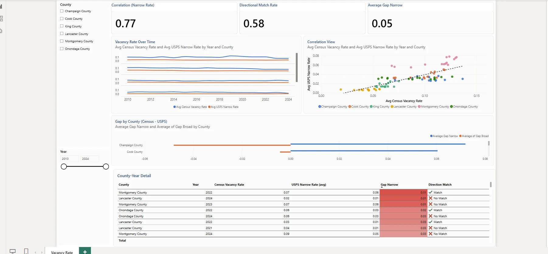
    Report overview: all six counties

    Nine visuals on one page: two slicers, three KPI cards, a small-multiples line chart, a scatter chart, a bar chart, and a county-year detail table.

    • KPI cards show the three answers at once: correlation (0.77), directional match rate (57.7%), and the average narrow gap.
    • Small multiples plot Census against USPS over time for each county, because a Power BI chart cannot legend by measure and by category at the same time.
    • The scatter chart with its trend line shows the counties sitting in different clusters, the first hint that one pooled number hides a lot.
    • The detail table flags, year by year, whether USPS moved in the same direction as Census.
  2. 2

    One county at a time

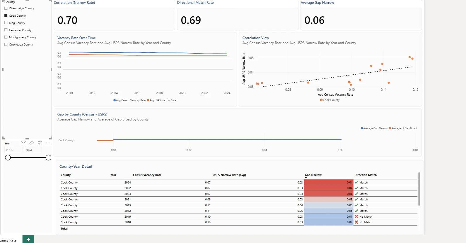
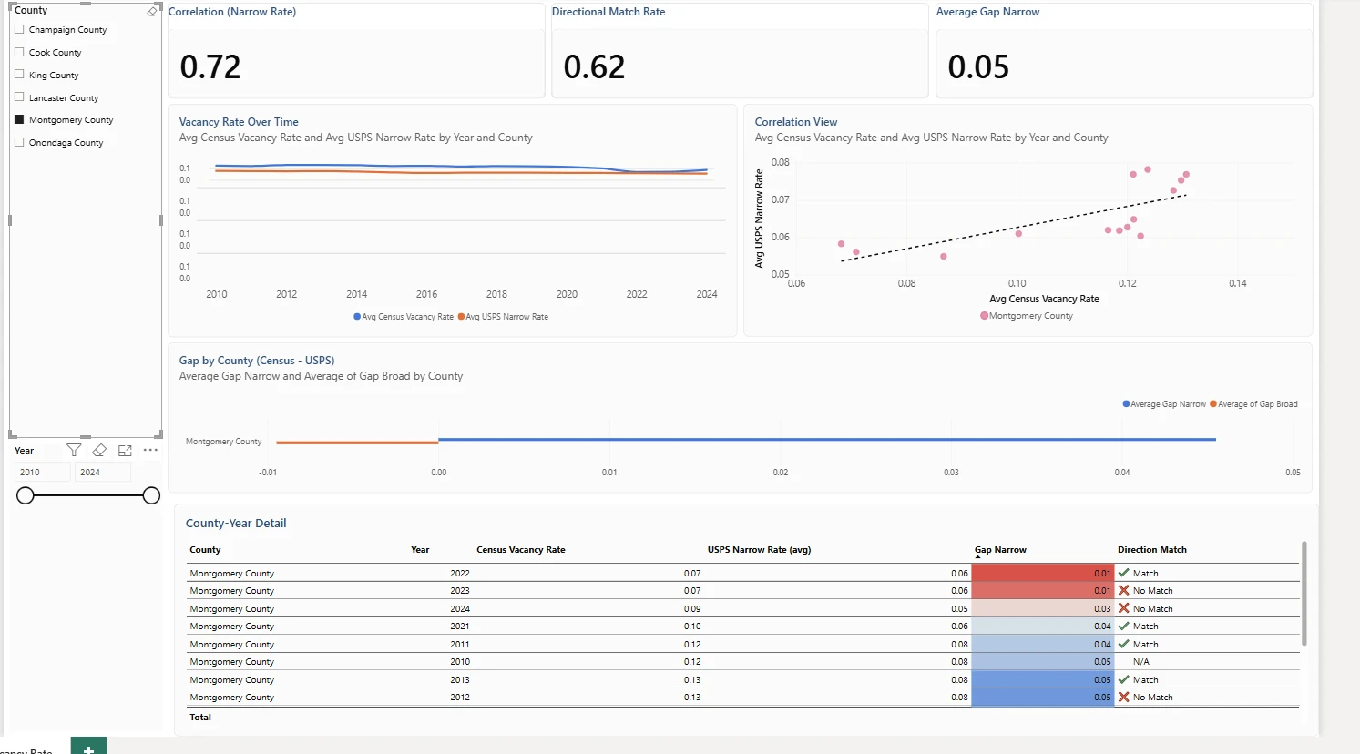
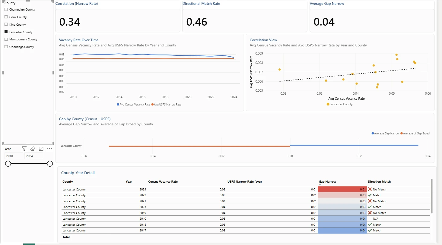
    Checking a single county recalculates every KPI and chart for that county alone, which is where the real story appears.

    • Montgomery, OH: r = 0.72 and Cook, IL: r = 0.70, where USPS tracks Census closely.
    • King, WA: r = 0.52, Lancaster, PA: r = 0.34, and Onondaga, NY: r = 0.26, which are weaker.
    • Champaign, IL: r = −0.01, no linear relationship visible in 14 county-years.
    • Conclusion: USPS tracks the Census level in some counties and not at all in others, and it called the direction right only 57.7% of the time, so it is a county-dependent signal at best (the follow-up nowcast project found no model beat last year’s number).
  3. 3

    The pipeline behind the dashboard

    Raw government files to a live report in five steps, all inside Microsoft Fabric.

    • Raw sources: USPS Vacant Address Report (quarterly, ZIP level) and Census ACS Table B25002 (annual, county).
    • Lakehouse: raw CSVs landed in USPS and Census folders, never edited.
    • Dataflow Gen2: combine quarterly files, roll up to county-year, join on FIPS and year, and fix two silent data-quality bugs.
    • Semantic model and report: calculated columns, DAX measures, slicers, KPI cards, and small multiples.
  4. 4

    Correlation by county

    The same pooled r of 0.77 breaks down very unevenly once you look county by county.

    • The spread from 0.72 down to −0.01 is why the project reports per-county results, not just the pooled figure.
    • This is the chart to show a stakeholder who asks whether they can rely on USPS for their county.
  5. 5

    Hand-built Pearson correlation in DAX

    DAX has no CORREL function, so the measure computes covariance and standard deviations with SUMX over the filtered rows.

    • Because it is a measure, it responds to every slicer, so each county's r is calculated live.
    • Every number it produces can be checked against the CSV with plain arithmetic.
Next projectGrocery Transaction Data Warehouse
Esc

↑ ↓ to moveEnter to open